Swarm Dynamics & Agent Based Modeling

This lesson has a little bit of something for everyone, and does not need to be done in sequence. Interested in mathematical modeling? Jump into Part A. Is simulation your thing? If so, hop to Part B. Are you in a gym full of friends who’ve all built BLIMPs? Part C will let you put your flying skills to the test.

---

Part A: Agent-based Swarm Model

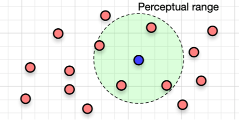
We will look at one of the most basic models that replicate collective motion of animal groups. The agents in the swarms are modeled as point masses that move around in the 2D or 3D space. Each agent can select its direction of motion based on the observed positions and velocities of the nearby agents. 

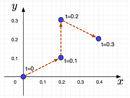
Time is partitioned into discrete time steps t, with a regular spacing of 0.1 s (corresponding to the response latency of the animal). We use c_i (t) to denote the position of agent #i at time t, and v_i (t) to denote its velocity vector at time t. The position is then updated according to the following equation:

c_i (t+0.1) = c_i (t) + 0.1 v_i (t).

Suppose agent #1 is initially at c₁ (0) = [0,0] in the xy-space, and suppose its trajectory is as shown in the figure below. What is the history of the velocities of this agent? 
Hint: v₁(0) = [2,1]. 
 v₁ (0.1)=  [      ,      ]      v₁ (0.2)= [     ,      ]       

The behavior of the agent is modeled by how the velocity vector is updated based on what it perceives. In the following, we will study basic rules that replicate animal group behaviors.

Repulsion / Collision Avoidance: We first consider how individuals attempt to always maintain a minimum distance between themselves and others. This rule has the highest priority and corresponds to a frequently observed behavior of animals in nature. 

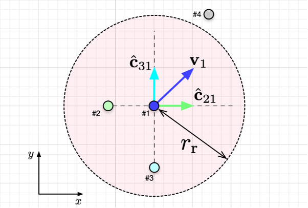
Each agent tries to move away from other agents within the range of r_r. This disk centered at the individual with radius r_r is called the “zone of repulsion” (ZOR), and the velocity vector will be updated according to

v_i(t+0.1)=Σ_jĉ_ji(t)

where ĉ_ji is a unit vector from agent i to agent j, and the summation is taken over all the neighbors that are in ZOR.  The following figure shows an example of the velocity vector v₁ that results from the repulsive behavior.  Observe how #1’s velocity is in the direction that moves away from #2 and #3.

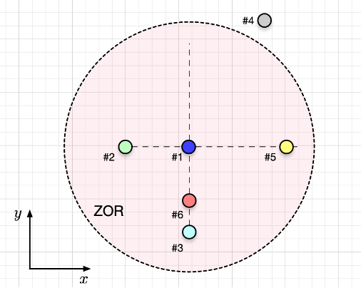
If there are two additional agents (#5 and #6), what will be the resultant velocity vector? Directly draw in the figure.

Let’s look at another example to further understand the repulsive behavior. Suppose agents #2 and #3 are fixed (they do not move) at coordinates [0, 0] and [0.8, 0], respectively.  We consider how agent #1, who is initially located at c₁(0)=[0.2, 0] with velocity v₁(0)=[0,0], moves in the next few time steps.  Assume that r_r=0.5 for this example.

Since the initial velocity is 0, the position at 0.1s is still c₁(0.1)=[0.2, 0]. Based on the repulsive behavior, the velocity vector at time 0.1s will be v₁(0.1)=[ ___, ___ ] m/s

Continuing the same process, find the position and velocity at time steps 0.2, 0.3, and 0.4:

• c₁(0.2)=______,    v₁(0.2)=______m/s
• c₁(0.3)=______,    v₁(0.3)=______m/s
• c₁(0.4)=______,    v₁(0.4)=______m/s

Observe that agent #1 will not move beyond 0.4 s.  This is because the virtual “repulsive forces” that drive the agent is balanced.  Such a state is called the “equilibrium.”

Orientation and Attraction: If individuals are not performing an avoidance maneuver, they tend to be attracted towards other individuals (to avoid being isolated) and to align themselves with neighbors. Specifically, if no neighbors are within the ZOR, the individual responds to others within the “zone of orientation” (ZOO) and the “zone of attraction” (ZOA).  These zones are circular / spherical except for a volume behind the individual.  This “blind volume” is defined as a cone with interior angle α.

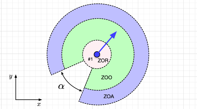
The ZOO starts outside of ZOR and ends at the distance r_o.  The ZOA starts outside of ZOO and ends at the distance r_a. An individual will attempt to align itself with neighbors within the zone of orientation and move towards the positions of individuals within the ZOA.  These two rules are added together as follows:

v_i(t+0.1)=0.5(Σ_jv̂_j(t)+Σ_jĉ_ji(t))

where v̂_j is the unit vector describing the direction of motion of agent #j.  The first summation is taken over all agents in the ZOO, and the second summation is over all agents in ZOA.  Note that ĉ_ji is the vector from i toward j which is the opposite of the one used for the repulsive behavior.

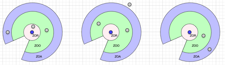
Identify which of the three behaviors (repulsion, orientation, and attraction) are active in the situations shown in the following figures.

Now that you understand some basic rules, let’s see how they work in computer simulation!

---

Part B: Collective Behaviors (Computer Simulation)

In the previous part, we saw how an individual reacts to the positions and velocities of other individuals in the group. In a multi-agent system, the collection of these local interactions results in a collective behavior of the group.  We will use computer simulation to see how the sizes of the behavioral zones affect the types of collective behaviors.

1. Follow the instructions linked here to create the simulation file “BLIMP_simulation.nlogo”.
2. Go to NetLogo Web
3. Find “Upload a Model” on the top right corner of the screen

4. Click on “Choose File” and navigate to the file you downloaded in step1
5. You should now see the BLIMP_simulation screen:

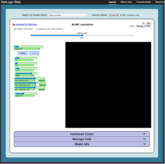
6. Click “setup” and then “go.” This will start the simulation.

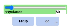
7. To change the population of the swarm, use the “population” slide bar, and don’t forget to hit “setup” again. You can play with this value, but the simulation will become slow if you increase the population too much.

We will now change the parameters r_a, r_o, and r_r to see how they affect the behavior of each individual as well as the behavior of the swarm as a whole. The meaning of these parameters is as follows:

• r_r is the radius of ZOR (r_r)
• r_o is the width of ZOO (r_o = Δr_o = r_o-r_r) 
• r_a is the width of ZOA (r_a = Δr_a=r_a-r_o)

Fragmenting: We will test how the parameters affect the “cohesiveness” of the swarm, i.e., how the agents can stay together.

• Set Δr_a=3, Δr_o=1, and r_r=1
• Run the simulation a few times and observe what happens to the swarm. (You can click on “setup” to restart the simulation from a new random position.)
• Increase the value of Δr_a and find the value for which the group always stays cohesive.

Phase transition: We will now see how the group exhibits different collective behaviors, and how that is dependent on the past. 

• Set r_r=1 and Δr_a=15.
• Set Δr_o=40. Run the simulation and describe the behavior. (You will probably see what’s called the “flocking” behavior.)
• Gradually reduce the value of Δr_o and observe how the behavior changes. 
• At what value of Δr_o did the behavior change? We’ll call this r_r1.
• Now, start from Δr_o=0 and increase it until you see the flocking again.
• At what value of Δr_o did you get the flocking? We’ll call this r_r2.

Notice how r_r1 and r_r2 are different. The switching in the behavior happens at different values of Δr_o depending on whether it was decreased from a higher value or increased from a lower value. This phenomenon is called the hysteresis.

Try different parameter settings and see if you can generate any “new” group behaviors! You can save the parameter values, take a screenshot and share it with us!

---

Part C: Collective Behaviors (BLIMPs)

Have you built a BLIMP yet? If so, you and a group of friends can try putting this into action! Try playing a game of aerial cat and mouse. Inflate a balloon with helium; we’ll call this balloon the cheese. Amongst your friends, pick one person to be the cat. The cat’s mission is to fly their BLIMP in a way to protect the cheese. Everyone else is a mouse, trying to fly their BLIMPs to get to the cheese without being attacked by the cat. Can the mice find a way to work collectively to get the cheese without being struck down by the cat?

---

Bonus

You can try many other Netlogo simulations (not necessarily related to swarms) from “Search the Models Library” at the top left menu.

Clicking on the “NetLogo Code” allows you to look at the code and even write your own.

You can learn more about it here: https://ccl.northwestern.edu/netlogo/docs/

---

Last updated June 24, 2022.